Open Source 1D/2D Inverse Laplace Program
Table of Contents
Author
Takahiro Ohkubo, Chiba university
https://amorphous.tf.chiba-u.jp/
Introduction
OSILAP (Open Source Inverse Laplace Program) is a program to solve 1D/2D inverse Laplace problem for NMR decay data. Butler-Reeds-Dawson algorithm is applied to decay data with non-negative constraint and regularization (smoothing) parameter \({\alpha}\). The distribution of \({T_1}\) (spin–lattice relaxation), \({T_2}\) (spin–spin relaxation), and \({D}\) (self-diffusion) are obtained from corresponding experimental decay data. Singular value decomposition of the decay data is employed to compress the kernel matrix and noise reduction as described in a paper (Venkataramanan et al.). The program is linked to the well-known linear algebra package LAPACK, efficient multithreading calculation is enabled to matrix operation.
Install
- An executable for Linux: osilap
- An executable for MacOS (intel): osilap
- An executable for MacOS (arm): osilap
- An executable for Windows: osilap.exe
- Build OSILAP from source: osilap-1.0.tgz
Execute OSILAP
OSILAP is a command line program, so you have to use "command prompt" on a windows box or "Terminal" on a MacOSX. An instruction movie may help this operation.
Prepare 1D/2D decay data
A 1D or 2D decay data is provided by a column-separated plain text file.
1D data
Header lines from the first "#" character onward are treated as comment and discarded. 1st and 2nd columns are time series in second and intensity in arbitrary unit, respectively. Number of lines corresponds to number of data points.
# CPMG cps data
#  time/s            I
0.002          810.754
0.004          694.388
0.006          589.836
0.008          515.479
0.010          447.298
0.012          393.103
.
.
.
2D data
The data size (X and Y) must be defined in the first line. The first column is additional time series (e.g. time increment of 180-90 pulse interval for inversion recovery). Second column is also time series (e.g. cumulative echo time in CPMG). Third column is intensity data. One data block with constant X is separated by two blank lines.
# X:100 Y:3000
0.001 0.00166667 -0.936219
0.001 0.00333333 -0.841772
0.001    0.005 -0.77891
.
.
.
0.001  4.99833 -0.00250787
0.001        5 -0.000563409


0.00110521 0.00166667 -0.934752
0.00110521 0.00333333 -0.835661
0.00110521    0.005 -0.770477
.
.
.
0.00110521  4.99833 -0.00299772
0.00110521        5 -0.00483022


0.00122149 0.00166667 -0.926351
0.00122149 0.00333333 -0.835368
0.00122149    0.005 -0.76921
.
.
.
Run OSILAP
OSILAP is run from only the command line with input file with command line options. The data dimension and data type must be explicitly passed in the command line. All command line options are listed. [\(value\)] is the default without explicit options.
command line options
\({\alpha}\) is the regularization parameter. In default, \({\alpha}\) is optimized to be balanced to noise. To determine \({\alpha}\), iterative calculation or S-curve method (developing) are applied to optimize \({\alpha}\). alpha_loop_max and alpha_tol are parameters to control iterative calculation. Scurve, Smin, Smax, Snum are the parameter for S-curve method. newton_loop_max and newton_tol are the parameters to control the convergence for Newton method.
Options:
 -i                      confirm calculation condition
 -h --help               show this help message
    --dimension=%d       one- or two-dimension [2]
    --alpha=%f           initial value of alpha (only BRD) [0.1]
    --sigma=%f           standard error, 0=auto [0.0]
    --sfactor=%f         sfactor for SVD [1e-4]
    --output=%s          basename of output file [basename]
    --TXspace=%s         TX space (log | linear) [log]
    --TXtype=%s          TX data type (T1 | T1inf | T1p | T2 | D) [T1]
    --TXmin=%f           TX minimum [0.0001]
    --TXmax=%f           TX maximum [10]
    --TXnum=%d           TX points [50]
    --TYspace=%s         TY space (log | linear) [log]
    --TYtype=%s          TY data type (T1 | T2 | D) [T2]
    --TYmin=%f           TY minimum [0.0001]
    --TYmax=%f           TY maximum [10]
    --TYnum=%d           TY points [50]
    --alpha_loop_max=%d  maximum iteration for alpha [5000]
    --alpha_tol=%f       alpha tolerance [1e-3]
    --newton_loop_max=%d maximum iteration for newton method [5000]
    --newton_tol=%f      newton tolerance [1e-8]
    --Scurve=%f          target for dlog10(chi)/dlog10(alpha) [0.0]
    --Smin=%f            search grid for s-curve [1e+6]
    --Smax=%f            search grid for s-curve [1e-6]
    --Snum=%d            search grid number for s-curve [20]
    --Atype=%d           calculation method of alpha for BRD routine [0]
Example 1: 1D CPMG (cpmg.int) with \({\alpha}\) optimization
\({\alpha}\) is optimized with iterative calculation.
osilap cpmg.int --dimension 1 --TXtype T2
Example 2: 1D CPMG (cpmg.int) with fixed \({\alpha=10^{-5}}\)
alpha_loop_max is set to 1. The initial \({\alpha}\) value is adopted for the analysis without \({\alpha}\) optimization.
osilap cpmg.int --dimension 1 --TXtype T2 --alpha 1e-5 --alpha_loop_max 1
Example 3: 2D Inversion-recovery-CPMG (ir-cpmg.int)
Execution of 2D inverse laplace transform with the default values.
osilap ir-cpmg.int
Output
Distribution data is saved in the file. It is noted that the listed intensity (\(I\)) is normalized by a normalized coefficient. To obtain absolute intensity, multiply \(I\) by the coefficient.
# -------------- solving condition -------------- #
#  sfactor:         1.000000e-04
#  initial alpha:   1e-05
#  alpha max loop:  1
#  alpha tol:       0.0001
#  Newton max loop: 5000
#  Newton tol:      1.000000e-08
#  A_opt method:    0
# --------------- TX information ---------------- #
#  Data space:      log
#  Data type:       T2
#  (TXmin, TXmax, TXpoints)=(0.0001, 10, 50)
# ------------------ input data ----------------- #
#  Input file:      example-1D/cpmg.int
#  Output basename: example-1D/cpmg
# ---------------- Compress data ---------------- #
#  K1 original :    999
#  K1 compress :    13
# ------------- Calculation results ------------- #
#  Alpha :          1.000000e-05
#  Sigma :          2.580453e+00
# ----------------------------------------- #

# Distribution normalized coeff.: 643.202
#            TX               I
 1.00000000e-04  0.00000000e+00
 1.26485522e-04  0.00000000e+00
 1.59985872e-04  0.00000000e+00
 .
 .
 .
Tools
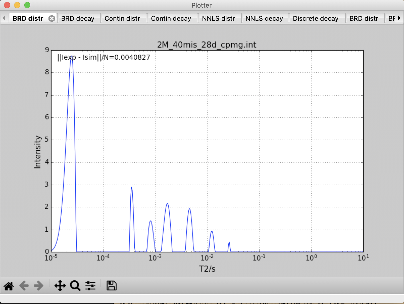
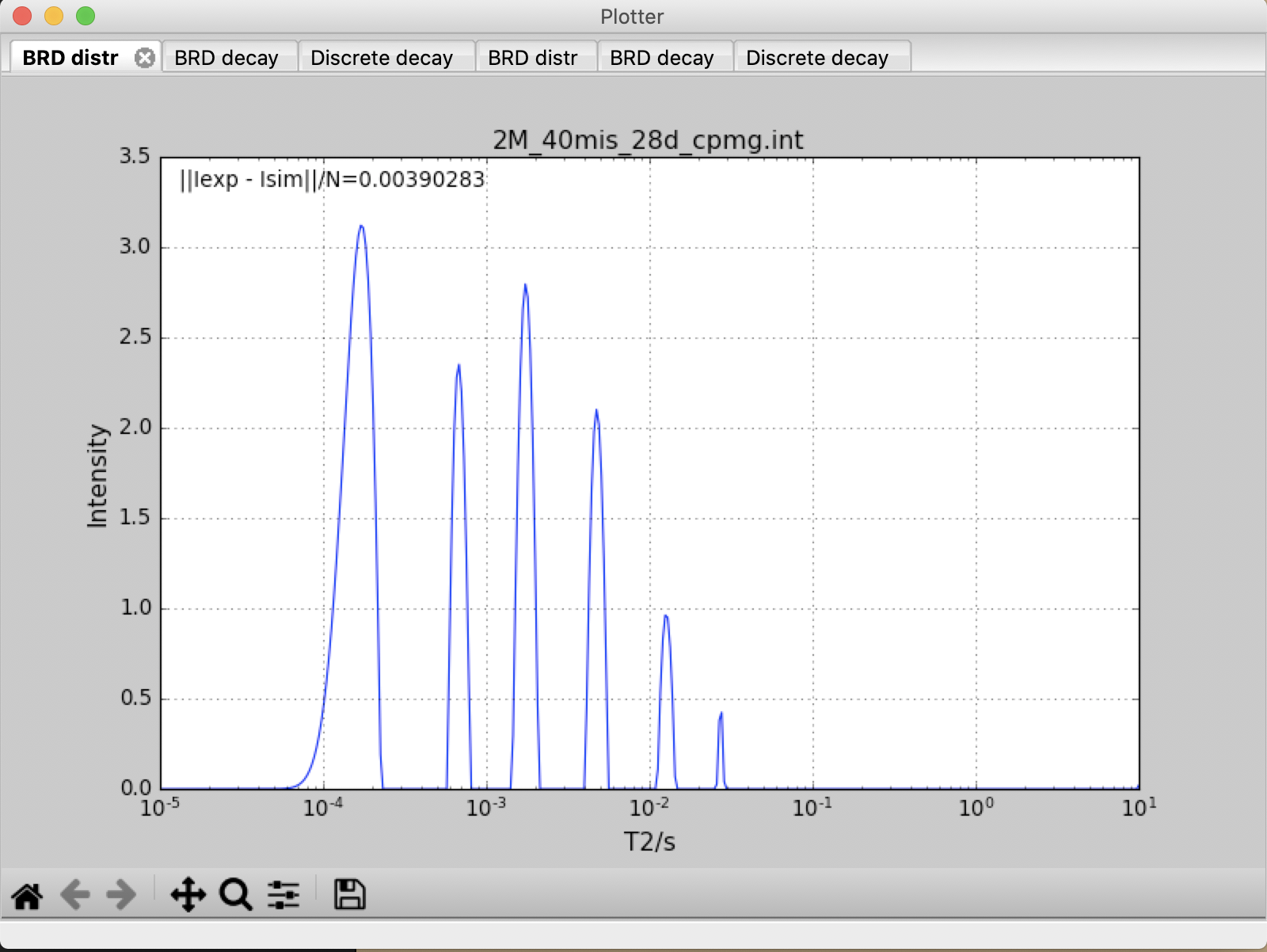
decay2distr.py
- download: decay2distr.py
decay2distr.py is a python program wrapping OSILAP for 1D data analyses. OSILAP is called with any options via subprocess module in python script. The program helps to run multiple input files and visualization of the results. Decay and resultant distribution data are immediately displayed on the screen using matplotlib and wxpython. DISCRETE (leastsq with \(n\) components), NNLS analyses using scipy module and CONTIN analysis are also applied to 1D decay data. Multiple files are sequentially analyzed with the same condition. This treatment is better to check the validity and compare all data. Resultant distribution data is saved in \(basename\).out as a textfile.
To run decay2distar.py, following modules are Required:
- numpy
- matplotlib
- scipy
- wxpython
Modified version from original CONTIN program is also required. The modified source and binary are redistributed under author's permission.
- An executable for Linux: contin
- An executable for MacOS (intel): contin
- An executable for MacOS (arm): contin
- An executable for Windows: contin.exe
- Build from source: contin_modify.tgz
Example 1:
- Input files are WC_31d.int and 2M_40mis_28d_cpmg.int.
- \(T_2\) distribution ranges between 0.000001 to 10.
- Number of points on \(T_2\) distribution is 400.
- \({\alpha}\) is fixed to 0.00001
decay2distr.py -x 1e-5 -y 10 -z 400 -alpha 1e-5 -alpha_loop 1 -f 2M_40mis_28d_cpmg.int WC_31d.int
Input file : 2M_40mis_28d_cpmg.int
Output file: 2M_40mis_28d_cpmg.out
------------------------------------------------------------------------
Analyzing BRD...
Analyzing CONTIN...
Analyzing NNLS...
Analyzing DISCRETE...

 ------------------------------------------------------------------------

Input file : WC_31d.int
Output file: WC_31d.out
------------------------------------------------------------------------
Analyzing BRD...
Analyzing CONTIN...
Analyzing NNLS...
Analyzing DISCRETE...

 ------------------------------------------------------------------------
All decay and distribution data are displayed on the screen, and saved in 2M_40mis_28d_cpmg.out and WC_31d.out as a text file..
Example 2:
- Same data and condition as Example 1:
- Avoid data with short time less than 0.0008
- Only OSILAP and discrete with 3 components analyses
decay2distr.py -x 1e-5 -y 10 -z 400 -alpha 1e-5 -alpha_loop 1 -f 2M_40mis_28d_cpmg.int WC_31d.int -s 0.0008 -m brd discrete -n 3
out2plot.py
- download: out2plot.py
out2plot.py is a program to display and integrate intensity for multiple out data. The thresholds to select integral ranges should be set.
WC_31d.out and 2M_40mis_28d_cpmg.out are passed to out2plot.py with integral boundaries at 0.0001, 0.001, and 0.003.
out2plot.py WC_31d.out 2M_40mis_28d_cpmg.out -b 1e-4 1e-3 3e-3
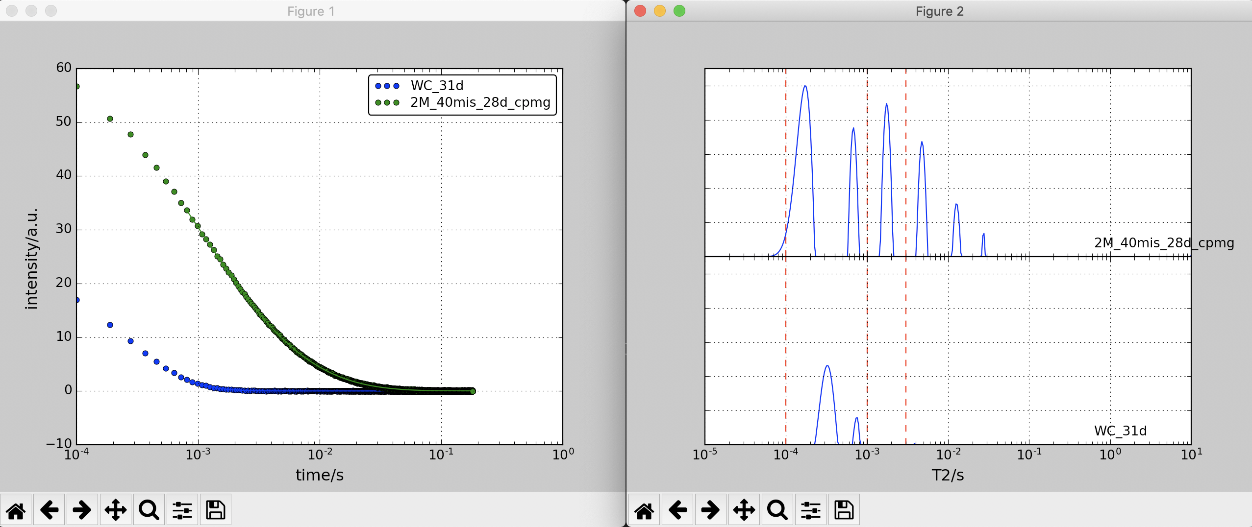
Results are displyed as follows:
# WC_31d.out (data type: brd)
1: [0,0.0001), [1e-05,9.82836e-05): 0.000716519 (0.00376966%)
2: [0.0001,0.001), [9.82836e-05,0.001): 18.9822 (99.8667%)
3: [0.001,0.003), [0.001,0.00302833): 0 (0%)
4: [0.003,1e+10), [0.00302833,10): 0.0246189 (0.129522%)
# 2M_40mis_28d_cpmg.out (data type: brd)
1: [0,0.0001), [1e-05,9.82836e-05): 1.18684 (1.18656%)
2: [0.0001,0.001), [9.82836e-05,0.001): 60.4243 (60.4099%)
3: [0.001,0.003), [0.001,0.00302833): 19.7965 (19.7918%)
4: [0.003,1e+10), [0.00302833,10): 18.6162 (18.6118%)
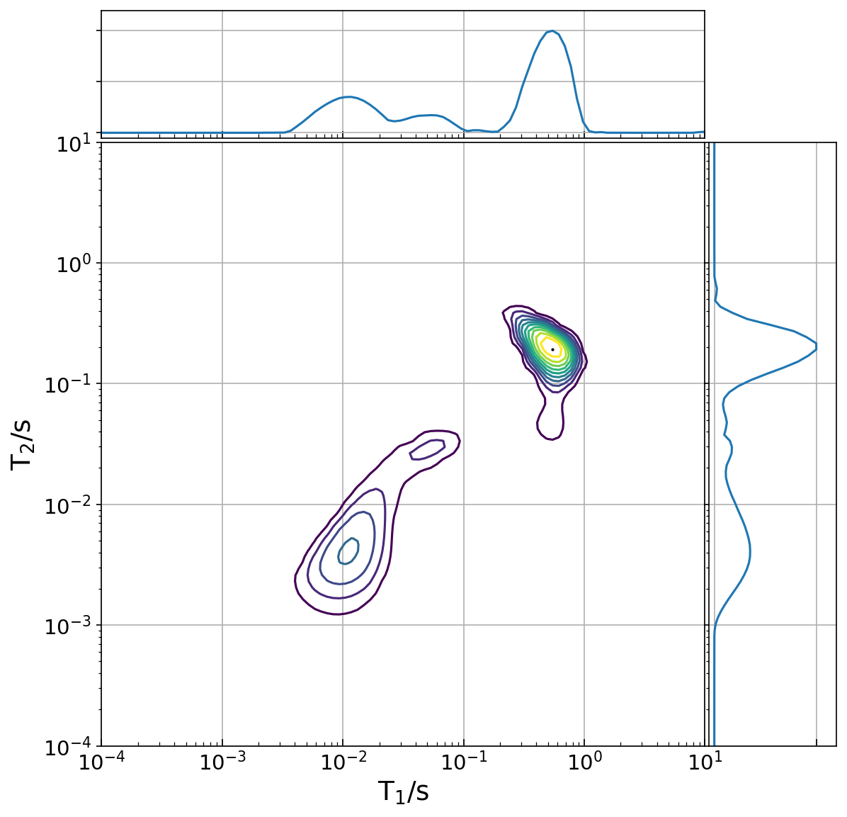
distrplot.py
- download: distrplot.py
distrplot.py is a contour plotter for *.distr file.
distrplot.py ir-cpmg.distr