Matplotlibの使い方
matplotlibは、データをプロットするためのライブラリです。データが大量に なってくると、数字を眺めていても何を意味しているのかわからないことがあ ります。実験やシミュレーションから出力される大量のデータを可視化するこ とで、データが示す意味を理解できるようになります。ビックデータを使った 新しい科学が注目を浴びているように、データの海から新しい価値を発掘 (data mining)するためにも可視化は重要です。
pythonから利用できる可視化用のライブラリは、データのタイプによっていく つかあります。2次元と3次元のデータをプロットするためのライブラリは、 matplotlibがもっとも普及しています。matplotlibは、2次元(\(x,y\) の データセット) と3次元データ(\(x, y, z\) のデータセット)を効率良く かつきれいに可視化することができます。matplotlib使った基本的な作図方法 を説明します。
注釈
4次元データは、(例えば電子密度のような \(|\psi(x, y, z)^2|\) のデータ)は、matplotlibでうまく表現できません。Mayavi等 (http://docs.enthought.com/mayavi/mayavi/) の可視化ライブラリを使う必要があります。
注釈
大学の計算機にインストールされているmatplotlibはversion 1.5.3です。 2018年1月現在、2.1.1が最新の安定versionです。1.5.x系から2.x系に version upすることで、デフォルトのスタイルが大きく変わっています。2.x 系で1.5.xと同じようなスタイルをプロットするためには、後述する plt.style.useで'classic'を指定します。
Matplotlibのインポート
matplotlibは、非常に多くのモジュール群で (https://matplotlib.org/py-modindex.html)構成されています。一般的の2次 元プロットを利用するだでけは、トップレベルのmatplotlibをimportする必要 なく、可視化するためのmatplotlib.pyplotのimportだけで十分です。
import matplotlib.pyplot as plt # (慣習)
プロットのスタイル
matplotlibは、デフォルトのプロットスタイルをスタイルシートという枠組み を使って好きに変えられます。デフォルトのスタイルを変更するためには、プ ログラムの先頭で以下のように定義します。
plt.style.use('classic') # 2.x系で1.5.x系のスタイルを使う
自分が使っているmatplotlibで利用できるスタイル一覧は plt.style.availableで得られます。
print(plt.style.available)
私のmacにインストールされているmatplotlib2.1.1の例です。
['_classic_test', 'bmh', 'classic', 'dark_background',
 'fivethirtyeight', 'ggplot', 'grayscale', 'seaborn-bright',
 'seaborn-colorblind', 'seaborn-dark-palette', 'seaborn-dark',
 'seaborn-darkgrid', 'seaborn-deep', 'seaborn-muted',
 'seaborn-notebook', 'seaborn-paper', 'seaborn-pastel',
 'seaborn-poster', 'seaborn-talk', 'seaborn-ticks',
 'seaborn-white', 'seaborn-whitegrid', 'seaborn']
スタイルを指定するために、py.style.use()を使います。
plt.style.use('classic')
初期設定
plt.style.use()で指定しない場合のデフォルトのスタイルは、環境設定ファ イルmatplotlibrcを使って指定することができます。自分用の環境設定ファイ ルを作っておけば、毎回設定する手間がはぶけて同じ体裁で作図することが可 能になります。matplotlibrcの配置場所は以下のとおりです。
プログラムと同じ場所にあるmatplotlibrc
ユーザのホームディレクトリの.matbolot/.matplotlibrc 自分の
matplotlibがインストールされているmpl-data
デフォルトを自分用のスタイルにしたい場合は、matplotlibがインストールさ れているmpl-dataの下のファイルをコピーして編集すれば良いでしょう。フォ ントのサイズや線幅等の細かい制御が可能になります。
matplotlibrcを変更を行わずに、プログラムの中からフォントサイズや線幅等 の変更を行うこともできます。
plt.rcParams.update({ 'legend.fontsize': 12, 'legend.numpoints': 1}
2次元プロット
\(x\) と \(y\) のリストを準備してplot()に渡せばプロットできます。
import matplotlib.pyplot as plt

x = [1, 2, 3, 4, 5, 6]
y = [1, 3, 5, 7, 9, 11]

fig, ax = plt.subplots()  # 図と軸の作成
ax.plot(x, y, "o-")       # 作成した軸にデータをプロット(点と線)
ax.set_xlabel('x axis')   # y軸のxラベル
ax.set_ylabel('y axis')   # y軸のyラベル
plt.show()                # 図の表示
numpyを使って関数プロットの方法について説明します。
import numpy as np
import matplotlib.pyplot as plt

x = np.linspace(0, 2*np.pi, 10) # 0から10まで100点のxデータ
y1 = (0.5*x)**2 # 0.1x^2のyデータ
y2 = np.sin(x) # sin(x)のyデータ
y3 = np.cos(x) # cos(x)のyデータ

fig, ax = plt.subplots() # 図と軸のオブジェクト生成
ax.plot(x, y1, "o", label="0.5**2") # 0.1x^2のプロット
ax.plot(x, y2, "s-", label="sin(x)") # sin(x)のプロット
ax.plot(x, y3, "--", label="cos(x)") # cos(x)のプロット
ax.set_xlabel("X") # Xラベル
ax.set_ylabel("Y") # Yラベル
ax.legend() # 凡例の表示
ax.set_xlim(0, 8)  # プロットのX範囲
ax.set_ylim(-2, 5) # プロットのY範囲
fig.savefig("test.png") # 図の保存

plt.show() # 図の表示
次のようなプロットが表示されtest.pngが保存されます。データの後に、マー カーの種類や線種、色を指定しています。またlabelで凡例に表示する文字列 を指定指定しています。
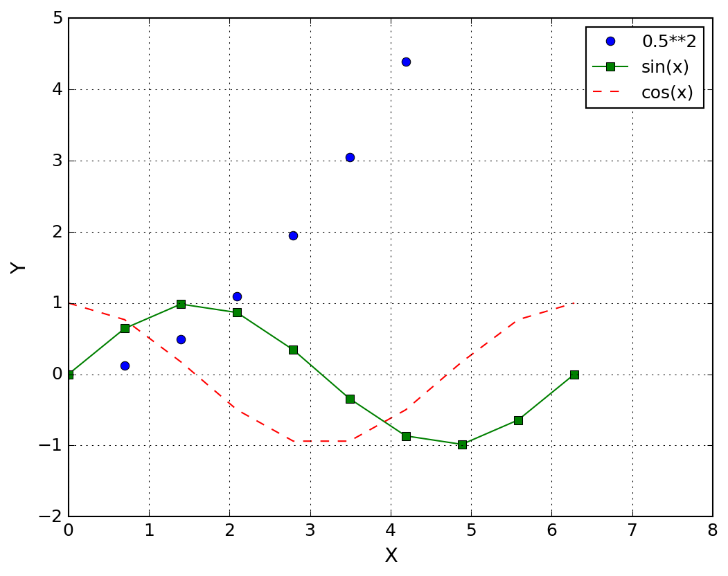
注釈
plt.plot(x, y)でプロットすることも可能ですが、「図」と「軸」のような オブジェクトを作成した方が、pythonらしいですし見通しが良いので、fig, とaxをplt.subplots()で作成しています。
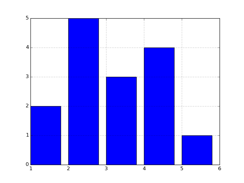
棒グラフプロット
barの位置と高さ、オプションで幅をbar()に渡せばbarプロットしてくれます。 barの位置は、barの'edge'か'center'のどちらか指定します。
import matplotlib.pyplot as plt

x = [1, 2, 3, 4, 5]
h = [2, 5, 3, 4, 1]
w = [0.8] * 5

fig, ax = plt.subplots()
ax.bar(x, h, width=w, align='edge')
fig.savefig('bar.png')
plt.show()
統計データは、ヒストグラムでプロットすると結果がわかりやすいです。デー タをpylab.histに渡すことでヒストグラムを作成できますが、numpyの histogramを使った方が自由にデータを処理ができるので、bins(区分)と hist(高さ)を計算してから、barでプロットすることとします。
https://matplotlib.org/devdocs/api/_as_gen/matplotlib.pyplot.bar.html
乱数て適当なデータを作ってプロットしています。
import numpy as np
import matplotlib.pyplot as plt

np.random.seed(7)
data =np.random.random(1000) * 10

hist, bins = np.histogram(data, bins=10) # 区分は等間隔で10分割
print(hist.size, bins.size) # 10と11
fig, ax = plt.subplots()
width = (bins[1:] - bins[:-1])     # 区分の幅
x = bins[:-1] + 0.5*width          # 区分の左側エッジ

plt.bar(x,  hist, width*0.8, align="center") # barの幅はwidthの80%

ax.set_xlabel("X")
ax.set_ylabel("Frequency")
fig.savefig("histogram.png")
plt.show()
以下のような図が得られます。
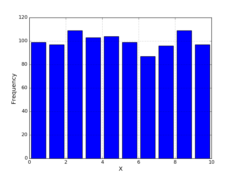
np.histogra()は、hist(高さ)とbins(区分のエッジ)を返しますが、bins.size はhist.sizeの+1になります。
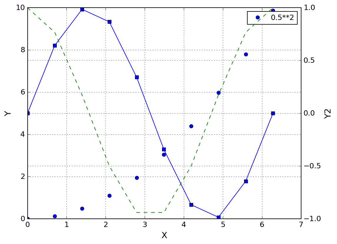
2軸でプロット
x軸を共有した2系統のデータをプロットしたい場合、X(またはY)軸を共有した いオブジェクトをax.twinx()(またはax.twiny())で作成してプロットします。
import numpy as np
import matplotlib.pyplot as plt

x = np.linspace(0, 2*np.pi, 10) # 0から10まで100点のxデータ
y1 = (0.5*x)**2 # 0.1x^2のyデータ
y2 = np.sin(x) # sin(x)のyデータ
y3 = np.cos(x) # cos(x)のyデータ
fig, ax = plt.subplots() # 図と軸のオブジェクト生成
ax.plot(x, y1, "o", label="0.5**2") # 0.1x^2のプロット
bx = ax.twinx()  # x軸を共有した新しい軸の生成
bx.plot(x, y2, "s-", label="sin(x)") # sin(x)のプロット
bx.plot(x, y3, "--", label="cos(x)") # cos(x)のプロット
ax.set_xlabel("X") # Xラベル
ax.set_ylabel("Y") # Yラベル
bx.set_ylabel("Y2") # Yラベル
ax.legend() # 凡例の表示
fig.savefig("twinx.png") # 図の保存
plt.show() # 図の表示
以下のような図が得られます。
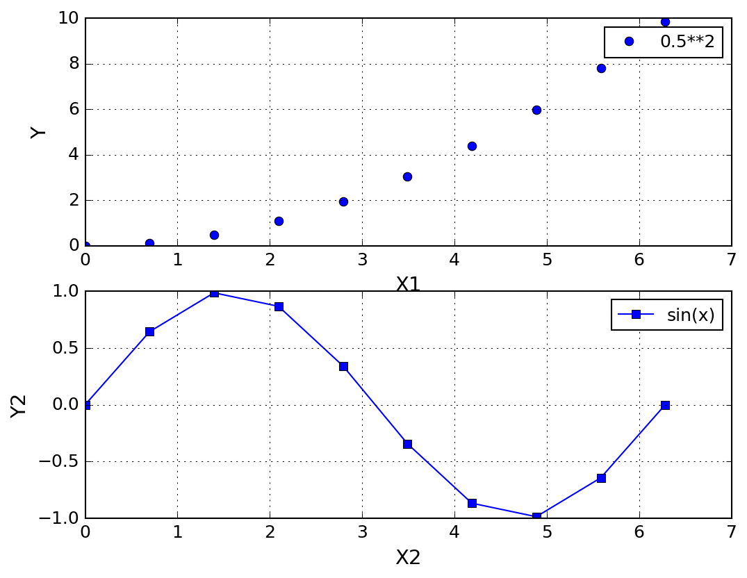
複数の図をプロット
plt.subplots()でfigとaxを生成する際、nrows, ncolsを指定することで図中 に複数の軸を配置させることができます。nrowsとncolsで複数の軸を生成した 場合、axは2次元配列になっています。プロットしたい軸のaxにplot()します。 またfigオブジェクトを複数生成すれば、複数の図を表示させることもできま す。
https://matplotlib.org/devdocs/api/_as_gen/matplotlib.pyplot.subplots.html
import numpy as np
import matplotlib.pyplot as plt
x = np.linspace(0, 2*np.pi, 10) # 0から10まで100点のxデータ
y1 = (0.5*x)**2 # 0.1x^2のyデータ
y2 = np.sin(x) # sin(x)のyデータ
y3 = np.cos(x) # cos(x)のyデータ
fig1, ax = plt.subplots(nrows=2, ncols=1) # 図と軸のオブジェクト生成
ax[0].plot(x, y1, "o", label="0.5**2") # 0.1x^2のプロット
ax[1].plot(x, y2, "s-", label="sin(x)") # sin(x)のプロット
ax[0].set_xlabel("X1") # Xラベル
ax[1].set_xlabel("X2") # Xラベル
ax[0].set_ylabel("Y") # Yラベル
ax[1].set_ylabel("Y2") # Yラベル
ax[0].legend() # 凡例の表示
ax[1].legend() # 凡例の表示
fig1.savefig("subplots-1.png") # 図の保存
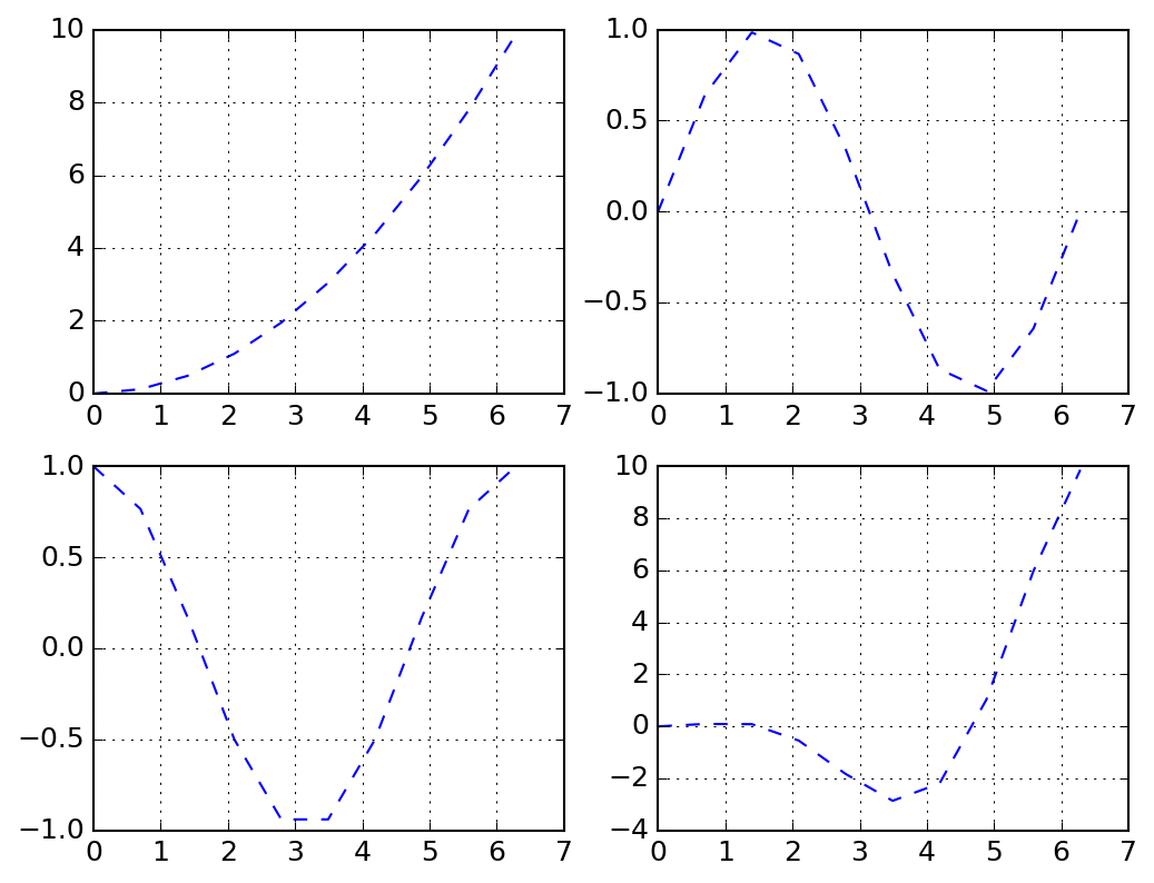
fig2, ax = plt.subplots(nrows=2, ncols=2) # 図と軸のオブジェクト生成
ax[0][0].plot(x, y1, "--") # (0, 0)
ax[0][1].plot(x, y2, "--") # (0, 1)
ax[1][0].plot(x, y3, "--") # (1, 0)
ax[1][1].plot(x, y1*y3, "--") # (1, 1)
fig2.savefig("subplots-2.png") # 図の保存
plt.show() # 図の表示
以下のような2つの図が得られます。
3次元プロット
3次元プロットは、3つのデータの組 \((x, y, f(x,y))\) を準備して可視 化します。データのパターンとして、 \((x, y)\) がグリッド(格子)上に 並ぶ場合と並んでいない場合の2パターンになります。
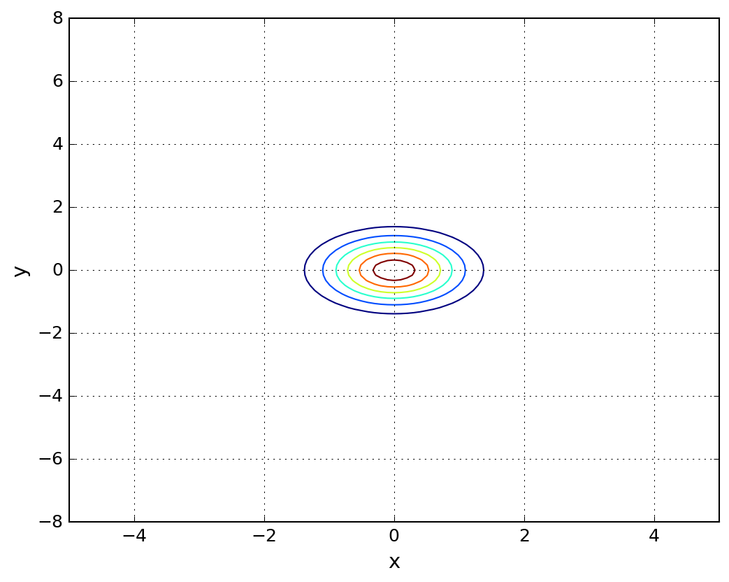
コンタープロット
xy平面上のグリッドの各点が値をもつようなデータのプロットによく用いられ ます。天気予報での気圧配置を思い浮かべると良いかと思います。100x50の格 子の場合、100x50の各格子点に対応する \(x\), \(y\), \(z\) のデータを準備します。格子状のデータを作成するために、np.meshgrid()が 便利です。
https://matplotlib.org/api/_as_gen/matplotlib.axes.Axes.contour.html
import numpy as np
import matplotlib.pyplot as plt

x = np.linspace(-5, 5, 101) # [-5.  -4.9 ... 5.0]
y = np.linspace(-8, 8, 101) # [-5.  -4.9 ... 5.0]
X, Y = np.meshgrid(x, y)
print(X)  # [[-5.  -4.9 -4.8 ...,  4.8  4.9  5. ]
          #  [-5.  -4.9 -4.8 ...,  4.8  4.9  5. ]
          #  [-5.  -4.9 -4.8 ...,  4.8  4.9  5. ]
          #  ...,
          #  [-5.  -4.9 -4.8 ...,  4.8  4.9  5. ]
          #  [-5.  -4.9 -4.8 ...,  4.8  4.9  5. ]
          #  [-5.  -4.9 -4.8 ...,  4.8  4.9  5. ]]
print(Y)  # [[-8.   -8.   -8.   ..., -8.   -8.   -8.  ]
          #  [-7.84 -7.84 -7.84 ..., -7.84 -7.84 -7.84]
          #  [-7.68 -7.68 -7.68 ..., -7.68 -7.68 -7.68]
          #  ...,
          #  [ 7.68  7.68  7.68 ...,  7.68  7.68  7.68]
          #  [ 7.84  7.84  7.84 ...,  7.84  7.84  7.84]
          #  [ 8.    8.    8.   ...,  8.    8.    8.  ]]

val = np.exp(-(X**2+Y**2))  # 2次元のガウス関数

fig, ax = plt.subplots()
ax.contour(X, Y, val)
ax.set_xlabel("x")
ax.set_ylabel("y")
fig.savefig("contour.png")
plt.show()
下のような図が得られます。
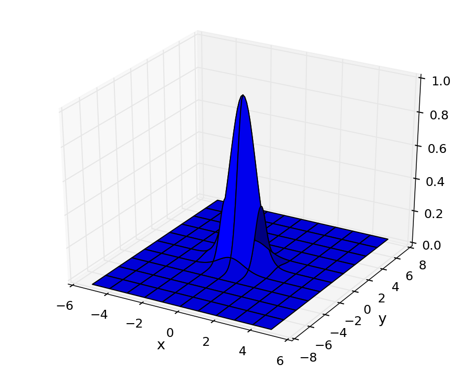
surfaceプロット
軸を3つとってデータを可視化したい場合、Axes3Dモジュールをimportしてプ ロットします。コンピュータの画面や紙は2次元ですので、奥行きを表現する 必要があります。いろんな3Dプロットの方法があります。
https://matplotlib.org/mpl_toolkits/mplot3d/tutorial.html#mplot3d-tutorial
ここでは1例として、球面調和関数の可視化に用いたsurfaceプロットだけ紹介 します。
https://matplotlib.org/mpl_toolkits/mplot3d/tutorial.html#surface-plots
import numpy as np
import matplotlib.pyplot as plt
from mpl_toolkits.mplot3d import Axes3D

x = np.linspace(-5, 5, 101) # [-5.  -4.9 ... 5.0]
y = np.linspace(-8, 8, 101) # [-5.  -4.9 ... 5.0]
X, Y = np.meshgrid(x, y)
print(X)  # [[-5.  -4.9 -4.8 ...,  4.8  4.9  5. ]
          #  [-5.  -4.9 -4.8 ...,  4.8  4.9  5. ]
          #  [-5.  -4.9 -4.8 ...,  4.8  4.9  5. ]
          #  ...,
          #  [-5.  -4.9 -4.8 ...,  4.8  4.9  5. ]
          #  [-5.  -4.9 -4.8 ...,  4.8  4.9  5. ]
          #  [-5.  -4.9 -4.8 ...,  4.8  4.9  5. ]]
print(Y)  # [[-8.   -8.   -8.   ..., -8.   -8.   -8.  ]
          #  [-7.84 -7.84 -7.84 ..., -7.84 -7.84 -7.84]
          #  [-7.68 -7.68 -7.68 ..., -7.68 -7.68 -7.68]
          #  ...,
          #  [ 7.68  7.68  7.68 ...,  7.68  7.68  7.68]
          #  [ 7.84  7.84  7.84 ...,  7.84  7.84  7.84]
          #  [ 8.    8.    8.   ...,  8.    8.    8.  ]]

val = np.exp(-(X**2+Y**2))  # 2次元のガウス関数
fig, ax = plt.subplots(subplot_kw={"projection": "3d"}) #プロット領域の作成

ax.plot_surface(X, Y, val)
ax.set_xlabel("x")
ax.set_ylabel("y")
plt.show()
下のような図が得られます。
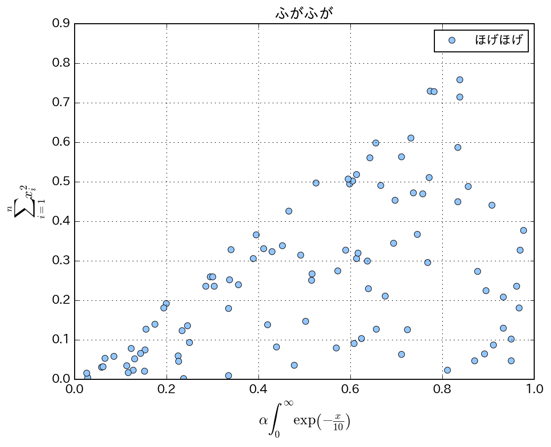
数式・日本語フォント
数式はlatexの数式モードの表記に従って記述します。latexは、洗練された組 版システム(図表をリファレンス等を割り付けてくれる)で、数式の表現が豊富 で美しいため、学術論文の作成によく使われます。テキストベースで数学記号
ギリシャ文字と数学記号の入力は下のURLを参照してください。
https://matplotlib.org/users/mathtext.html#symbols
いくつか例を上げます。括弧はペアで配置しないとエラーになります。分数は frac{}{} で表記します。以下の数式をxlabelとylabelに割り付けてみます。
日本語を表示させるためには、日本語用フォントを準備せねばなりません。OS のfont置き場にあるttfフォントを指定します。当然ですが、日本語のttfフォ ントでなれば日本語は表示できません。日本語を含むフリーのttfフォントを ダウンロードして利用していみます。
https://ipafont.ipa.go.jp/old/ipafont/download.html
ipaexg.ttf(ゴシックフォント)をシステムのフォント置き場に移動します。 windowsの場合はC:WindowsFonts、macの場合は/LibraryFonts等です。後は Pythonのプログラムでフォントの名前をfont.familyにセットすれば日本語が 使えます。
import numpy as np
import matplotlib as mpl
import matplotlib.pyplot as plt
import matplotlib.font_manager as font_manager

# デフォルトのスタイルを変えてプロット
plt.style.use('seaborn-pastel')

# フォントの配置場所にあるttfフォントを指定
path = '/Users/takahiro/Library/Fonts/ipaexg.ttf'
# フォントのプロパティ
prop = font_manager.FontProperties(fname=path)
# フォントの名前を取得
mpl.rcParams['font.family'] = prop.get_name()

x = np.random.random(100)
y = np.random.random(100) * x
fig, ax = plt.subplots()
xl = r'$\alpha\int_0^{\infty}\exp\left( -\frac{x}{10} \right)$'
yl = r'$\sum_{i=1}^n x_i^2$'
ax.plot(x, y, "o", label="ほげほげ")
ax.set_xlabel(xl)
ax.set_ylabel(yl)
ax.set_title('ふがふが')
ax.legend()
fig.savefig("japanese-font.png")
plt.show()